Portfolio Optimization Problem

Which portfolio is the best?

This question is probably as old as the stock-market itself.

People spend a lot of time developing methods and strategies that come close to the "perfect investment", that brings high returns coupled with low risk.

As one of the most important and influential theories dealing this problem, Modern Portfolio Theory was developed by Harry Markowitz and published under the title "Portfolio Selection" in the 1952 Journal of Finance.

Let's review some math!

• \(m\) risky assets: \(i= 1, 2, \dots, m\)
• Single - Period Returns: \(\mathbf{R} = [R_{1,t}, R_{2,t}, \dots, R_{m,t}]^T\)
• Return calcualated from price: \(R_{1,t} = \frac{R_{1,t}-R_{1,t-1}}{R_{1,t-1}}\)
• Mean (Expected Returns) and Variance/Covariance of Returns: \[ E[\mathbf{R}] = \mathbf{\alpha} = \begin{bmatrix} \alpha_1 \\ \vdots \\ \alpha_m \end{bmatrix} , \quad \text{Cov}[\mathbf{R}] = \mathbf{\Sigma} = \begin{bmatrix} \Sigma_{1,1} & \cdots & \Sigma_{1,m} \\ \vdots & \ddots & \vdots \\ \Sigma_{m,1} & \cdots & \Sigma_{m,m} \end{bmatrix} \]
• Portfolio: \(m\) weights indicating the fraction of portfolio wealth held in each asset, \(\mathbf{w} = [w_1, \dots, w_m] : \, \sum^m_{i=1} = 1\) (fully invested)

• Portfolio Return: \[R_\mathbf{w} = \mathbf{w}^T \mathbf{R} = \sum^m_{i=1} w_i R_i\] \[\alpha_{\mathbf{w}} = E[R_{\mathbf{w}}] = \mathbf{w}^T \mathbf{\alpha}\] \[ \sigma^2_{\mathbf{w}} = \text{var} [R_{\mathbf{w}}] = \mathbf{w}^T \Sigma \mathbf{w}\]

• People are risk averse, we evaluate different portfolios using the mean-variance pair of the portfolio: \((\alpha_{\mathbf{w}},\sigma^2_{\mathbf{w}} )\) with preference for:

  • Higher expected return \(\alpha_{\mathbf{w}}\)
  • Lower variance \(\text{Var}_{\mathbf{w}}\), or its square root \(\sigma_{\mathbf{w}}\), standard deviation

Risk Minimization:

For a given choice of target mean return \(\alpha_0\), choose the portfolio \(\mathbf{w}\) to

Solution:

Apply the method of Lagrange multipliers to the convex minimization problem subject to linear constrains, we can get optimal portfolio weights and variance.

Matrix operation steps: Check reference [3]

Based on this problem, my project is to build and backtest strategies for 8 selected stocks since 2006.

Expected Return Maximization:

For a given choice of target return variance \(\sigma_0^2\), choose the portfolio \(\mathbf{w}\) to

Risk Aversion Optimization:

Let \(\lambda \geq 0\) denote the Arrow-Pratt risk aversion index gauging the trade-off between risk and return. Choose the portfolio \(\mathbf{w}\) to

There are many other popular problems involved with more complicated constrains. My project is an application of Problem 1 - Risk Minimization.

Import closing stock price data from Yahoo Finance from 01/01/2006 to 03/31/2016.

• Select following 8 stocks

• Code is reproducible for different total number, different date range and different companies of stocks chosen

• Objective: Minimize Portfolio volatility given a 15% annual return target

• Porfolio will be fuly invested (sum of weights = 1)

• Long Short is allowed ( weights between 200% and -200% )

• Portfolio is weekly rebalanced

Note: all parameters are replaceable in the code

Expected Returns

Historic returns are often used to estimate expecetd returns

• Sample Estimator for daily returns with 60 days of observation for expected returns.

Covariance Candidates are:

• Sample Covariance with 200 days of observation for returns, configuration referred as "long term", "long" or "l"

• Sample Covariance with 120 days of observation for returns, configuration referred as "medium term","medium" or "m"

• Sample Covariance with 60 days of observation for returns, configuration referred as "short term", "short" or "s"

Note: all parameters are replaceable in the code

library(rJava); library(tseries); library(quadprog) 
library(PerformanceAnalytics); library(ggplot2)
library(xlsx); library(data.table);library(xtable)

JPM <- get.hist.quote(instrument="JPM", start="2006-01-01", end="2016-3-31", quote="Close")
GOOGL <- get.hist.quote(instrument="GOOGL", start="2006-01-01", end="2016-3-31", quote="Close")
DIS <- get.hist.quote(instrument="DIS", start="2006-01-01", end="2016-3-31", quote="Close")
JCP <- get.hist.quote(instrument="JCP", start="2006-01-01", end="2016-3-31", quote="Close")
JNJ <- get.hist.quote(instrument="JNJ", start="2006-01-01", end="2016-3-31", quote="Close")
SBUX <- get.hist.quote(instrument="SBUX", start="2006-01-01", end="2016-3-31", quote="Close")
XOM <- get.hist.quote(instrument="XOM", start="2006-01-01", end="2016-3-31", quote="Close")
HOT <- get.hist.quote(instrument="HOT", start="2006-01-01", end="2016-3-31", quote="Close")


price_raw <- cbind(JPM, GOOGL, DIS, JCP, JNJ, SBUX, XOM, HOT)

Daily Returns

return_daily <- diff(price_raw)/lag(price_raw, k=-1)
colnames(return_daily) <- c("JPM", "GOOGL", "DIS", "JCP", "JNJ", "SBUX", "XOM", "HOT")

# head(return_daily, 4)

n1 <- nrow(return_daily)
n2 <- ncol(return_daily)
return_daily <- cbind(return_daily, portfolio=rep(NA,n1))
weight <- matrix(NA, nrow = n1, ncol = n2)
i = 1 + 60  # short: i = 1 + 60 
             # medium: i = 1 + 120
             # long:i = 1 + 200
             # If you don't want to observe from 2006-01-04
             # change 1 to b <- which(format(index(return_daily), "%Y-%m-%d") == '2008-01-05'

while (i <= n1){
  return_expect <- colMeans(return_daily[(i-60):(i-1), 1:n2], na.rm=TRUE) 
          # 60 days of observation for expected returns, fixed in my project, can change if you desire different estimator
  Dmat <- cov(return_daily[(i-60):(i-1), 1:n2], use = "complete.obs") 
          # Sample Covariance with 60 days of observation for returns, change to m: 120; l: 200
  Amat <- cbind(1, return_expect, diag(1,n2), diag(-1,n2))
  target <- 0.15 / 250
         # target yearly return 15%, fixed in my project, can change if you desire different constrain
  bvec <- c(1, target, -2+rep(0,n2), -2+rep(0,n2))
  dvec <- rep(0,n2)
  opt_sol <- solve.QP(Dmat,dvec,Amat,bvec, meq=2, factorized=FALSE)$solution
         # solve the optimization problem
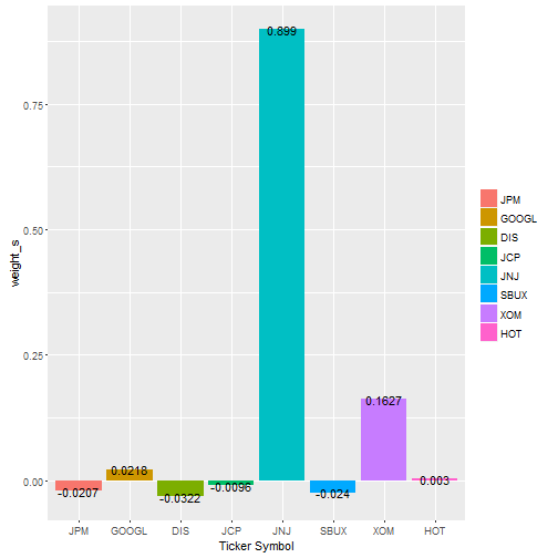
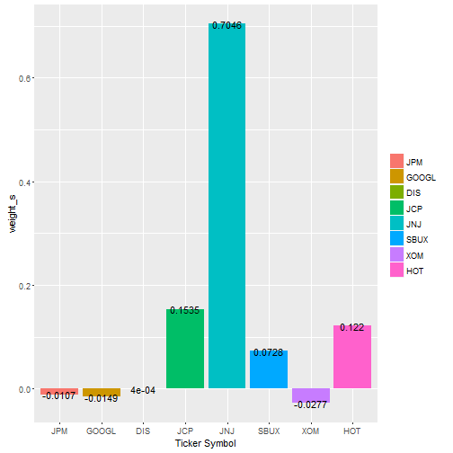
  weight[i+0:min(4,n1-i), ] <- matrix(rep(opt_sol, min(5,n1-i+1)), ncol=n2, byrow=T)
         # record weight for each asset
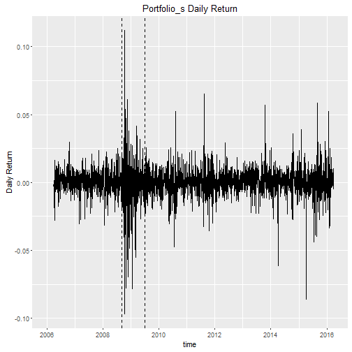
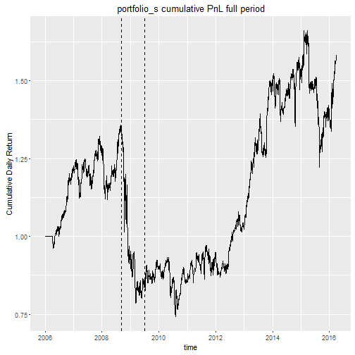
  return_daily[i+0:min(4,n1-i), n2+1] <- return_daily[i+0:min(4,n1-i), 1:n2] %*% opt_sol
         # record new daily return for each asset and portfolio overall
  i = i + 5 
         # weekly rebalance portfolio, adjust weight per 5 trading day
         # fixed in my project, can change if you desire different condition
}

• Record new daily return for each asset and portfolio overall

daily_s <- return_daily

# tail(daily_s,2)

• extract portfolio daily return

portfolio_s <- return_daily[,"portfolio"]

• record weight for each asset

weight_s <- data.frame(weight)
rownames(weight_s) <- as.character(index(daily_s))
colnames(weight_s) <- colnames(daily_s)[1:8]

In the following page, we will check our global setting:

1. full investment: sum of the weight = 1

2. portfolio is weekly balanced

Fully invested: sum of weight = 1

sum(weight_s[100,1:8])

## [1] 1

sum(weight_s[200,1:8])

## [1] 1

weight adjusted every five days

# tail(weight_s, 9)

Pick some dates to visuaize weight under each stock on a particular date

• can change to the following "2008-09-15" to any trading day

weight_s <- setDT(weight_s, keep.rownames = TRUE)[]
bar <- subset(weight_s, rn == "2008-09-15")
bar_melt <- melt(bar, id.vars="rn")

ggplot(bar_melt, aes(x=variable, y=value)) + 
  geom_bar(stat="identity", position = "identity",aes(fill=variable)) +
  geom_text(aes(x=variable, y=value, label=round(value, digits = 4))) +
  labs(x="Ticker Symbol",y="weight_s") +
  theme(legend.title=element_blank())

• 2008-09-15： when Lehman Brothers filed bankruptcy

• 2015-12-16： when Fed Raises Key Interest Rate for First Time in Almost a Decade

autoplot(daily_s$portfolio[1:2577], main="Portfolio_s Daily Return", facets=NULL) + 
    xlab("time") + ylab("Daily Return") + 
    geom_vline(xintercept=as.numeric(index(daily_s[c(674,879),])), linetype="dashed")

Some observations:

• During crisis period (2008-2010), return volatility is much lager than usual.

• For a extreme volatility in one day, it is usually caused by company splitted its stock, the price became half instantly

Graphs about daily return is not natural, investors feel comfortable to look at Cumulative PnL (returns)

Record Cumulative returns

cummu_s <- daily_s
for (j in 1:n1)
  cummu_s[j, ] <- apply(daily_s[1:j, ], 2, Return.cumulative) + 1

autoplot(cummu_s$portfolio[1:2577], main="portfolio_s cumulative PnL full period", facets=NULL) + 
      xlab("time") + ylab("Cumulative Daily Return") +
     geom_vline(xintercept=as.numeric(index(cummu_s[c(674,879),])), linetype="dashed")

Now we can apply the same methods by using medium and long term estimator.

Recall:

• Sample Covariance with 200 days of observation for returns, configuration referred as "long term", "long" or "l"

• Sample Covariance with 120 days of observation for returns, configuration referred as "medium term","medium" or "m"

• Sample Covariance with 60 days of observation for returns, configuration referred as "short term", "short" or "s"

cummu <- cbind(cummu_s[,"portfolio"], cummu_m[,"portfolio"], cummu_l[,"portfolio"])
colnames(cummu) <- c("short","mediam","long")



cummu <- data.frame(cummu)
cummu_date <- setDT(cummu, keep.rownames = TRUE)[]
cummu_melt <- melt(cummu_date, id.vars="rn")
cummu_melt$rn <- as.Date(cummu_melt$rn)

Is it the end of our story?

• Crisis:

  • Begin of the crisis: 2008 Sep 7, The Federal Housing Finance Agency (FHFA) places Fannie Mae and Freddie Mac in government conservatorship. A week later, Lehman Brothers filed bankruptcy.
    
  • It ended in June 2009, according to the U.S. National Bureau of Economic Research (NBER)

• data set (return_daily)

  • Before crisis: return_daily[,1:674]
  • During crisis: return_daily[,675:878]
  • After crisis: return_daily[,879:1512]

• Nobody evaluates a portfolio by is just looking at the cumulative PnL

library(xtable)
print(xtable(report_b,digits=5), type = "html")

• Short-term estimator works the best

  • highest daily return: closest to 15% target
  • annualized Shape Ratio is greater than 1

• volatility

  • medium estimator has smallest volatility
  • volatility from short estimator is about the same

• medium and long term estimator work better than short

  • medium estimator has highest return: though it is negative, far from our target
  • long term estimator has smallest volatility
  • medium estimator has better result in Shape Ratio, Sortino ratio and Maximum Drawdown

• Note: the portfolio during crisis has negative return.

• Long-term estimator works the best
  • highest daily return
  • lowest volatility
  • better result in Shape Ratio and Sortino ratio

• Same estimation method would have different performances under different market enviroment.

• When I write the code, I tried to make it more reproduceble; you may simply change/add/remove the ticker symbols, change the number of days for estimators, or adjust the time period, to create your own portfolio and visualization.

• Next step:

  • Maybe a shiny app ?
  • Make expected return estimator fancier: currently I am using return in previous 60 trading days to estimate, this naive attempt can be replaced by many other techniques

1. http://www.investopedia.com/articles/06/mpt.asp#ixzz4B2w779uJ
2. http://www.efalken.com/LowVolClassics/markowitz_JF1952.pdf
3. http://ocw.mit.edu/courses/mathematics/18-s096-topics-in-mathematics-with-applications-in-finance-fall-2013/lecture-notes/MIT18_S096F13_lecnote14.pdf